This is a collection of tutorials that show how to use the R.ROSETTA package.

Installation

Installation from github requires devtools package:

install.packages("devtools")

Installation and loading R.ROSETTA package from github:

library(devtools)
install_github("komorowskilab/R.ROSETTA")
library(R.ROSETTA)

Input format

The input is a decision table in a form of data.frame, where the columns represent features and rows represent objects. In the table last column shall contain the decision classes.
Decision table format
feature_1 feature_2 feature_n outcome
object_1 case
object_2 control
object_3 case
object_n case

To deal with complex decision tables we suggest to use feature selection methods.


Sample data

Synthetic

You can create a synthetic decision table with predefined correlation. Let’s assume that we want to create a decision table with 100 objects and 20 features that level of feature-feature correlation is 0.4 and the level of feature-decision correlation is 0.6. In this example the outcome is balanced and has two decision classes. To generate such data, type:

dt <- synData(nFeatures=20, rf=0.4, rd=0.6, nObjects=100, nOutcome=2, unbalanced=F, seed=1)

Now we add double correlated features at the level of 0.1 and 0.7, and triple correlated features at the level of 0.8 and 0.2. We will set up feature-feature correlation as a constant number 0.5. We set numeric vectors as the parameters, the order of nFeatures and R vectors must correspond to each other:

dt <- synData(nFeatures=c(20,2,2,3,3), rf=c(0.5,0.5,0.5,0.5,0.5), rd=c(0.5,0.1,0.7,0.8,0.2), nObjects=100, nOutcome=2, unbalanced=F, seed=1)

Gene expression

The package contains gene expression dataset from case-control studies for autism prediction. Decision table exists as a data.frame named autcon.

dt <- autcon

Running data

The main function to run a classifier is rosetta(). The default parameters of the function are set for the processing of the sample datasets. To display the parameters type the help function ?rosetta.

Continuous

To create rough set-based model from continuous data, type:

# synthetic data
dt <- synData(nFeatures=c(20,2,2,3,3), rf=c(0.1,0.1,0.1,0.8,0.8), rd=c(0.5,0.1,0.7,0.8,0.2), nObjects=100, nOutcome=2, unbalanced=F, seed=1)
out_s <- rosetta(dt)

# gene expression data
out_ge <- rosetta(autcon)

As you may notice, the default parametrs are set towards processing of continuous data.

Discrete

If your decision table contains all discrete features please use option discrete=TRUE. Here is an example of processing synthetic data with discrete values:

dt <- synData(nFeatures=c(5,5,3,2,2), rf=c(0.2,0.3,0.2,0.4,0.4), 
               rd=c(0.2,0.3,0.4,0.5,0.6), discrete = T, levels = 3, labels = c("low", "medium", "high"))
outd <- rosetta(dt, discrete = T)

Mixed

For data containing a mixture of continuous and discrete features, please use option discrete=FALSE and assign following object type to the features:

  • Continuous features that require discretization: numeric
  • Discrete features: character, factor, logical
dt <- synData(nFeatures=c(20,2,2,3,3), rf=c(0.1,0.1,0.1,0.8,0.8), rd=c(0.5,0.1,0.7,0.8,0.2), nObjects=100, nOutcome=2, unbalanced=F, seed=1)

# change two of the feature from the group 5 to discrete
dt$f5.2_rf0.8_rd0.2 <- as.factor(cut(dt$f5.2_rf0.8_rd0.2,3, labels = c("low", "medium", "high"))) # or as.character
dt$f5.3_rf0.8_rd0.2 <- as.factor(cut(dt$f5.3_rf0.8_rd0.2,3, labels = c("low", "medium", "high"))) # or as.character
out <- rosetta(dt, discrete = F)

Output

The rosetta() function generates two main outputs. The rule table is stored as a data.frame structure under $main. The model quality is stored as a table structure under $quality.

Main

The main output of the function contains a collection of rules in a table. The rule components and all statistics values are collected in separate columns. The individual values are comma separated.

dt <- synData(nFeatures=c(20,2,2,3,3), rf=c(0.2,0.2,0.3,0.5,0.5), rd=c(0.5,0.1,0.7,0.8,0.2), nObjects=100, nOutcome=2, unbalanced=F, seed=1) 
out <- rosetta(dt)
out$main
Main output
features levels decision support accuracy coverage cuts statistics
rule_1 F1,F2 1,2 case 43 0.97 0.174
rule_2 F2,F4,F5 2,1,3 control 40 0.95 0.142
rule_3 F2 3 case 36 0.89 0.097
rule_n F7,F1 3,1 control 10 0.64 0.014
  • features - attribute names from a rule
  • levels - discretization levels corresponding to a features
  • decision - decision class for a rule
  • accuracy - rule accuracy, for RHS(Righ Hand Support)
  • support - the number of objects supporting the rule, RHS(Righ Hand Support) or LHS(Left Hand Support)
  • coverage - rule coverage, RHS(Righ Hand Support) or LHS(Left Hand Support)
  • cuts - information about cuts (thresholds) used for discretization. This will not exist if we use discrete=T option.
  • statistics - rule p-values, risk ratios and confidence intervals for a rule.
Quality

Estimated accuracy and AUC values are collected into table. The values are taken from n-fold Cross-Validation process.

dt <- synData(nFeatures=c(20,2,2,3,3), rf=c(0.1,0.1,0.7,0.7,0.7), rd=c(0.5,0.1,0.7,0.8,0.2), nObjects=100, nOutcome=2, unbalanced=F, seed=1)
out <- rosetta(dt)
out$quality
Model quality
accuracyMean accuracyMedian accuracyStd accuracyMin accuracyMax
0.85 0.9 0.12693 0.6 1

If you need an information about AUC, please take look at the code below:

dt <- synData(nFeatures=c(20,2,2,3,3), rf=c(0.1,0.1,0.7,0.7,0.7), rd=c(0.5,0.1,0.7,0.8,0.2), nObjects=100, nOutcome=2, unbalanced=F, seed=1)
out <- rosetta(dt, roc = TRUE, clroc = "D1")
out$quality
Model quality
accuracyMean accuracyMedian accuracyStd accuracyMin accuracyMax ROC.AUC ROC.AUC.SE
0.85 0.9 0.12693 0.6 1 0.68 0.176738
ROC.AUC.MEAN ROC.AUC.MEDIAN ROC.AUC.STDEV ROC.AUC.MIN ROC.AUC.MAX ROC.AUC.SE.MEAN
0.9055 1 0.146358 0.625 1 0.060934
ROC.AUC.SE.MEDIAN ROC.AUC.SE.STDEV ROC.AUC.SE.MIN ROC.AUC.SE.MAX
0 0.082205 0 0.185339

Recalculate model

R.ROSETTA allows to recalculate a model according to the input decision table. This step may be used to retrieve a statistics in case of performing undersampling.

Let’s consider that one of our rules has support 24 and accuracy 0.92. These values come from a model that was divided into smaller training sets in the process of balancing the data. Thanks to the model recalculation we obtain support 32 and accuracy 0.95, which now are the values corresponding to the input decision table. To recalculate a model, run recalculateRules():

dt <- synData(nFeatures=c(20,2,2,3,3), rf=c(0.1,0.1,0.7,0.7,0.7), rd=c(0.5,0.1,0.7,0.8,0.2), nObjects=100, nOutcome=2, unbalanced=F, seed=1)
out <- rosetta(dt)
rules <- out$main
newRules <- recalculateRules(dt, rules)

Additionally model recalculation calculates support sets, which are added as the last columns in the data.frame object. ***

Plot rule

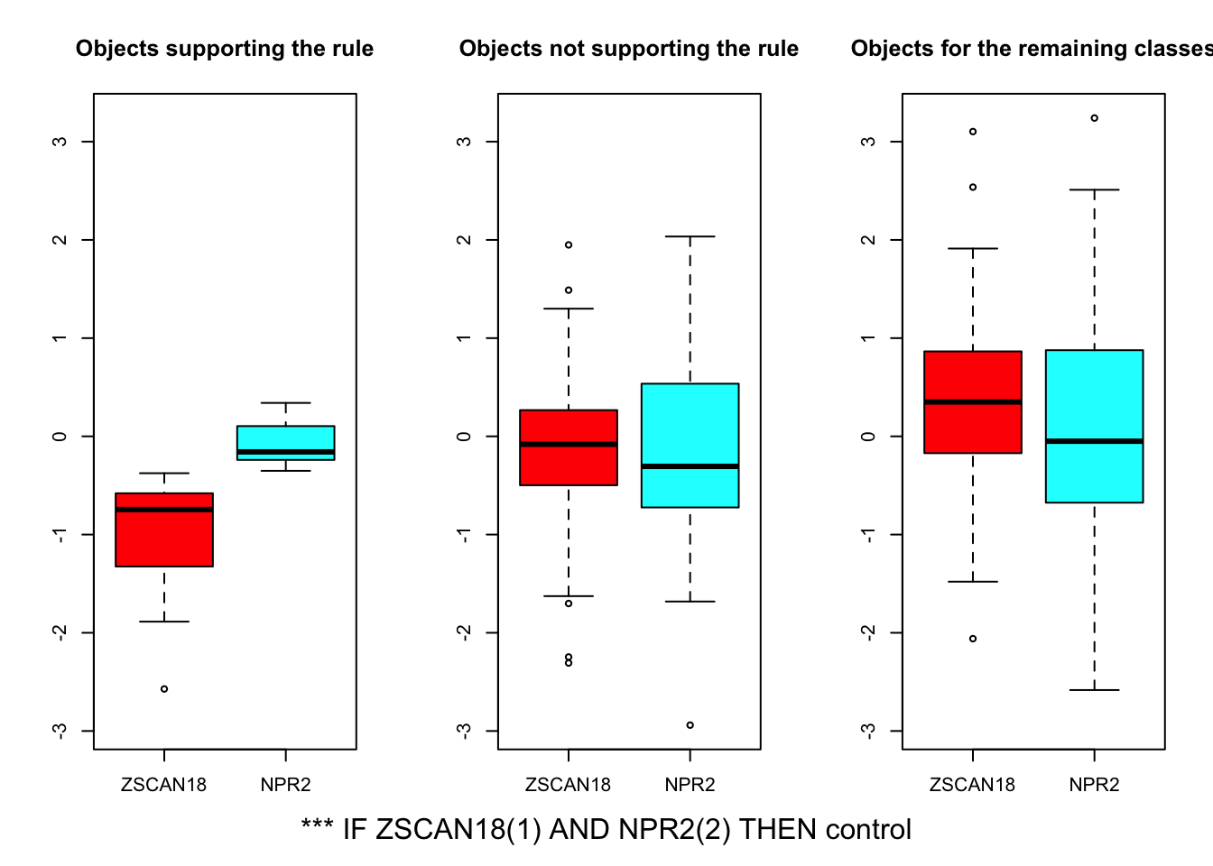
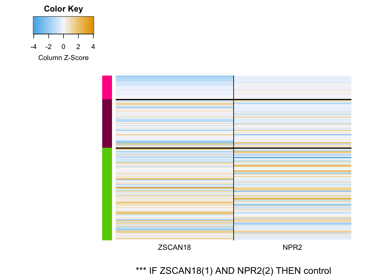
We can visualize a specific rule in a form of heatmap or boxplot. The plot presents a distribution of values for three support groups. This visualization is done only after recalculating the model.

out <- rosetta(autcon)
rules <- out$main
newRules <- recalculateRules(autcon, rules)
#rule heatmap
plotRule(autcon, newRules, type = "heatmap", ind = 1)

#rule boxplot
plotRule(autcon, newRules, type = "boxplot", ind = 1)


Predict unseen data

To test your model on external data you may use the predictClass() function. The algorithm validates if the levels of discretization correspond to the external dataset. Make sure that feature names correspond to the names used in the model.

### continuous data

## 1. to create a model
dt1 <- synData(nFeatures=c(20,2,2,3,3), rf=c(0.1,0.1,0.7,0.7,0.7), rd=c(0.5,0.1,0.7,0.8,0.2), nObjects=100, nOutcome=2, unbalanced=F, seed=1)
## 2. to validate the model (less objects, different seed, the same outcome)
dt2 <- synData(nFeatures=c(20,2,2,3,3), rf=c(0.1,0.1,0.7,0.7,0.7), rd=c(0.5,0.1,0.7,0.8,0.2), nObjects=50, nOutcome=2, unbalanced=F, seed=2)
#store decision
dt2_decision <- dt2$decision
#remove decision from table
dt2 <- dt2[,-length(dt2)]

out <- rosetta(dt1)
rules <- out$main

# we can predict new classes if we don't have the outcome
predictClass(dt2, rules)
# if the outcome is known, we can obtain the accuracy of external prediction
predictClass(dt2, rules, validate = TRUE, defClass = dt2_decision)

### discrete data
dt1 <- synData(nFeatures=c(20,2,2,3,3), rf=c(0.1,0.1,0.7,0.7,0.7), rd=c(0.5,0.1,0.7,0.8,0.2), nObjects=100, nOutcome=2, unbalanced=F, discrete=T, levels=3, labels=c("LOW","MEDIUM","HIGH"), seed=1)
## 2. to validate the model (less objects, different seed, the same outcome)
dt2 <- synData(nFeatures=c(20,2,2,3,3), rf=c(0.1,0.1,0.7,0.7,0.7), rd=c(0.5,0.1,0.7,0.8,0.2), nObjects=50, nOutcome=2, unbalanced=F, discrete=T, levels=3, labels=c("LOW","MEDIUM","HIGH"), seed=2)
#store decision
dt2_decision <- dt2$decision
#remove decision from table
dt2 <- dt2[,-length(dt2)]

out <- rosetta(dt1, discrete = T)
rules <- out$main

# we can predict new classes if we don't have the outcome
predictClass(dt2, rules, discrete = T)
# if the outcome is known, we can obtain the accuracy of external prediction
predictClass(dt2, rules, discrete = T, validate = TRUE, defClass = dt2_decision)